MohammedAmin.com
Serious writing for
serious readers

Search this site

Custom Search

Very early in one's training for any financial profession (for example training as a chartered accountant) one encounters the time value of money, discounting cash flows, and the concept of the internal rate of return.

Very briefly, if you specify:

1. A series of future cash flows which are received at future points in time, whether you count them all in future days, future weeks, future months or future years, where "C_t" is the cash flow arising at time t. The cash flow C_t may be negative (by convention used to represent investments that you make which require spending cash such as buying a share or building a factory) or positive (when the investment pays you a return such as a dividend, income from the factory, or sale proceeds.)
2. A rate "r" for discounting future cash flows. This discount rate can differ from period to period, but for convenience in practice most calculations are done with a discount rate which is the same for all periods.
3. With "n" as the number of equally spaced time periods under consideration. (A cash flow does not need to arise at each time period.)

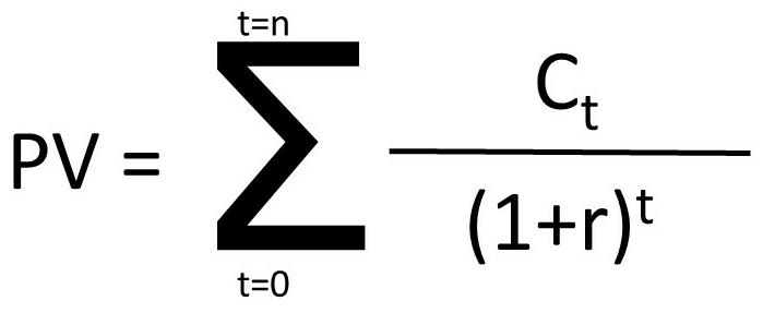
Then the present value of the series of future cash flows, PV, is computed as follows:

PV = C₀/(1+r)⁰ + C₁/(1+r)¹ + C₂/(1+r)² +... (and so on) ... C_n/(1+r)ⁿ

or in more concise mathematical notation:

Numerical illustration of discounting

Consider the following cash flows:

Here there is one single investment of 400 at time 0, followed by 10 positive cash receipts. If one discounts this series of cash flows at 5% per period, the arithmetic is as follows:

The table below shows each mathematical formula, copied from the Excel spreadsheet which is used for all of these workings.

Here $A$3 references the Excel spreadsheet cell A3 which holds the discount rate "r"of 0.05 which is of course 5%.

A6, A7 etc are the successive values of time "t" in the formula given earlier on the page.

Internal rate of return

Discounting needs you to specify a rate (or rates if you have different discount rates for different periods) that you will use to discount the cash flows. In the above example, 5% was your choice. You could equally well have discounted at 4%, 9% or any other rate you chose.

Obviously the higher the discount rate, the lower the aggregate NPV since higher discount rates reduce the positive cash flows in periods 1 - 10 to smaller NPV numbers.

An obvious question to ask is, is there a discount rate which results in calculating an aggregate NPV of zero?

That depends on the cash flow pattern. If all of the cash flows were positive (i.e. there was no initial -400 at time 0, only the positive receipts from times 1-10), then with any finite discount rate, no matter how large, the aggregate NPV is always greater than zero. Only an infinite discount rate will produce a zero NPV, if all cash flows are positive, and even then only if there is no positive cash flow at time 0.

With the cash flows in the example, one can calculate the discount rate that produces an aggregate NPV of zero. In the Excel spreadsheet you can repeatedly change cell A3 until the total NPV becomes zero. To four decimal places, a discount rate of 12.2816% makes the total NPV equal to zero. Instead of trial and error, one can use the Excel goal seeking tool, which is how I calculated 12.2816%.

This discount rate, which makes the NPV = 0 is known as the internal rate of return, or "IRR".

In the above equation, the IRR is the value of "r" for which NPV=0, if such a value exists. In other words, it is the value of "r" that solves the equation:

0 = C₀/(1+r)⁰ + C₁/(1+r)¹ + C₂/(1+r)² +... (and so on) ... C_n/(1+r)ⁿ

For values of t up to 4, there are general solutions to the above equation, since the equation can be rewritten in the form

0 = A + Br + Dr² + Er³ + Fr⁴ where A, B, D, E, F are computed by multiplying out the divisors in the previous equation and then rearranging the terms.

However that does not guarantee that there is a value of r that solves the equation. Even with simple quadratic equations, of the form 0 = A + Bx + Cx² we know from school algebra that there may be no real solutions. As mentioned before, if all cash flows are positive, there will be no finite IRR.

For values of t greater than 4, there is no general solution, since in the nineteenth century Abel proved there was no algebraic solution to the general quintic polynomial equation.

Instead of having to use goal seeking, Excel contains a function which I have in the past found very useful, which computes the IRR for you. Its format is as follows. In the cell where you want the IRR to be shown, type:

=IRR ([range of cash flow values in a horizontal or vertical line, with the periods equally spaced],[a guess to get Excel's calculation started])

Its usage is shown in the spreadsheet extract below:

Financial concerns with the internal rate of return

Those receiving a financial education are taught to consider the pros and cons of using IRR or NPV to evaluate projects, and in general to prefer the use of NPV for a number of reasons which are outside the scope of this article.

One point which is often validly made is that the mathematics will generate multiple values for the IRR. Very briefly, in general, for every sign reversal in the cash flows (where a negative cash flow is followed by a positive cash flow, or a positive cash flow is followed by a negative cash flow) one potentially generates another solution value.

In the above numerical example, with only one sign reversal, (-400 followed by solely positive cash flows) there was a unique value of "r" as the solution, with r = 0.1228 (i.e. 12.28%). However more complicated cash flow sequences with more sign reversals may generate several IRR values; all of them are as real as each other. Being conservative, one normally uses the lowest computed IRR value in such cases.

A more serious problem with Excel

The spreadsheets I build for myself normally compute NPV rather than IRR. However for decades I have regularly used the Excel IRR function, and regarded its outputs as reliable. Accordingly I had a shock last month.

I was performing a simple calculation. A few years ago, I bought an investment for £7,962.64, received a dividend of £157.32, bought some more of the same investment for £2,310.24, received some more dividends, and still own the investment. (The identity of the investment is not disclosed, because I do not wish to be exposed to the risk of giving investment advice.)

I wanted to see how the investment was performing, by computing the monthly IRR. (The cash flows occur more frequently than annually.) The monthly IRR_m can easily be converted to an annual IRR_a using the following formula:

1 + IRR_a = (1 + IRR_m)¹²

The cash flows are set out on the "Investment" tab of the spreadsheet and reproduced below:

The investment is still owned, so the 29 December 2016 cash flow is the dividend received in December 2016 plus the market value of the investment at 29 December 2016.

I then used the Excel IRR function to calculate the monthly IRR, and was delighted to see a monthly IRR of 4.9% which equates to an annual IRR of 78.4%. However a moment's look at the cash flows, which only show a total undiscounted gain of £3,048.40 shows that the annual IRR could not possibly be 78.4%.

When in doubt with a calculation, it helps to perform it more simply, without relying upon complicated formulas. Accordingly, I set up a calculation in the form of a bank account simulation, as shown by the table below:

Here one starts by making the investment of £7,962.64, with all positive cash flows being shown as withdrawals from the bank account, and extra investments shown as additions to the bank account. The specified rate of return is then the interest that the "bank" is deemed to pay on the net cash invested into it, i.e. your "net investment in the account."

With a specified monthly rate of return of 1%, the closing value after deducting the 29 December 2016 cash flow from the dividend and notional market value sale, is £313.52. That shows that 1% is a good guess at the monthly rate of return, but is slightly too high since there is allegedly something left over after you have taken everything out of the investment.

Again, using the Excel goal seeking tool, one can easily compute that a monthly return of 0.9181% leaves you with a terminal value of exactly zero. This corresponds to an annual rate of return of 11.6% which is by no means spectacular, but is much better than doing nothing or losing money.

In the linked spreadsheet, on the "Investment" tab, I have set out the calculation giving rise to the spurious Excel calculated monthly IRR of 4.9%. Using that to discount each of the individual cash flows shows that one does not get an NPV of zero. Conversely when the true internal rate of return of 0.9181% is used to discount the cash flows, the NPV is indeed zero as expected.

I could not understand why Excel's IRR function was giving such ridiculous answers. I have used IRR often in the past, and found it to generate reliable results.

Explanation

A chance discussion with one of my sons, who is a computer programmer, found the explanation. It illustrates how frustrating computers and their logic can be.

In my past uses of the IRR function, the cash flows I have been working with have usually been calculated from other numbers on the spreadsheet. Accordingly, every cell in the range of cash flows is either non-zero (an actual cash flow) or zero (representing the total of some cells that add to zero.)

However in the case of this investment, since the cash flows only occurred on certain dates, I simply pasted the cash flows on those dates into column B on the tab "Investment". The other cells in column B were left blank.

However, Excel does not treat those blank cells as if they contained a zero. Instead, the cell, and the row the cell is on, are ignored in the IRR calculation.

This is explained in more detail on the spreadsheet's "Explanation" tab. That tab has three sections.

Base case calculations

This simply repeats the calculations on the "Investment" tab leading to the spurious IRR of 4.9% per month.

Excel has treated the blank cells as if they did not exist. Accordingly it has calculated actually IRR for the set of cash flows below.

In this section, I have deleted the rows that had blank cells. That is how the Excel IRR function is seeing the data. After deleting the rows with blank cells, I understood why Excel was calculating a 4.9% per month IRR. With a very short period of time for the investment to generate the dividends and final capital value, a very high IRR is necessary.

If in the original set of cash flows, zero is inserted in the cells where no cash flow arises, Excel sees the correct spacing of the periods and then computes a correct IRR

This section reproduces the cash flows on the investment.

However here an explicit "0" is typed into each cell when there is no cash flow. Excel's IRR function now sees the cash flows with their true spacing over time, and now computes the correct IRR of 0.9181%.

Concluding comments

Having had this experience, I will ensure that in future there are never any blank cells in a range if I am computing the IRR of that range of cash flows.

This is problem I have never encountered in several decades of using Excel, which is why I have written this page to share the experience.